Stock price analysis using Python with Pandas Library and SQL

Karl Chong
Apr 9, 2022
8 min read

Updated: Apr 10, 2022

Introduction:

Canada Inflation Rate - https://tradingeconomics.com/canada/inflation-cpi

Canada’s annual inflation rate rises to 5.7% in February of 2022, the highest since 1991. The inflation is getting higher and higher not only in Canada, but this is also the global trend. Although inflation will affect company’s sales and earnings, it is still more important than ever to invest in the stock market because invested in equities is one of the good ways to stay ahead of inflation. The question is: which stock to invest in 2022? Is there any fast and easy way to analyze and pick stocks? There are few stocks in my mind that worth investing but I want to know which one is “better”. The goal for this blog is to perform stocks analysis with Pandas and related libraries in Python so that I can pick the “winning” stock base on data.

The analysis will base on historical data and performance, only concerning the price change. The other criteria such as market share, earning reports are not considered. To improve the efficiency, I am going to write a simple “Analyzing Program” to speed up the process. The stocks I am going to analyze and compare are Tesla, Apple, Nvidia, Shopify and Bank of America. In the end I wish to create a program that can perform the analysis task on any stock.

P.S. This is a second blog extending the content from blog 1 - I highly recommend you to go through blog 1 before reading blog 2.

P.S. The "Today" mentioned in the blog is referring to "2022-4-8"

All the demo code can be found at: https://github.com/ckskarl/Blog2StockAnalysis

Which stocks and which criteria am I going to compare?

I have picked the following stocks to join the “arena”:

Company (Ticker)	Company Description	Reason for picking the company
Tesla(TSLA)	Pioneer in Electric Car and Battery Industry	Why not? We love Papa Elon :D
Apple (AAPL)	The largest IT company by revenue	Great eco-system + Huge Hardware & Software Profit
Nvidia (NVDA)	Dominating in GPU Market	High “Computing Demand” = High Profit
Shopify (SHOP)	Leading E-commerce SaaS company	One of the famous Canada Tech Company
Bank of America (BAC)	American multinational investment bank and financial services holding company	“Traditional” Finance Stock, I am expecting a much lower risk in inverting it

Before I start, Let’s have a look on some stock data from Yahoo Finance (e.g. Nvidia vs Shopify)

Both stocks seem to be performing well, but how should I quantify the performance? There are four criteria I would like to compare ( I will calculate my custom “Weighed Score” with the following weighing factor, base on my personal risk-reward preference):

Criteria	Description	Weighing Factor
Return since 2022-1-1 (%) (YTD Return)	Year-To-Date (YTD) return is the amount of profit (or loss) by an investment since the first trading day of the current calendar year. It can be the hint of how “sensitive” the company is to recent increase in inflation rate.	15
Return since 2017-4-8 (%) (5 Year Return)	The investment return received for a 5-year period; I would also include the dividends in the calculation. It represents the long-term performance.	5
Max Return (%) (5 Year)	The max return during the 5-year period; it uses the max price of a stock in the 5-year period compare with the price at day1. It represents the “growth” of the company. The greater the value, the faster growth of the company	1
Max Drawdown (%) (5 Year)	A maximum drawdown (MDD) is the maximum observed loss from a peak to a trough of before a new peak is attained. It is an indicator of downside risk over the 5-year. They play a huge impact on your compounding abilities. Huge drawdowns might force you to stop trading, it even might lead to ruin, and it makes your returns lower.	30
Weighed Score	The weighed sum of the 4 other criteria

For example:

Ticker	YTD Return	5 Year Return	Max Return (5Year)	Max Drawdown (5years)	Weighed Score
test	10	20	300	-40	(1015)+(2005)+(3001)+(-4030) =250

Then the one with the highest weighed score is the “winner”.

Part A - Getting historical stock prices and Calculating criteria

First I will be using Pandas data reader to get price data from Yahoo Finance. We need to import three libraries:

import pandas_datareader.data as web
import datetime
import pandas as pd

If you haven’t installed the corresponding package, you can install them by following:

1. View -> Tool Window-> Python Packages -> search the library name -> click install

2. pip install: (https://pip.pypa.io/en/stable/cli/pip_install/)

Pandas Datareader is a Python package that allows us to create a pandas DataFrame object by using various data sources from the internet. It is popularly used for working with realtime stock price datasets.

The following code snippet will get Tesla’s price data from Yahoo Finance, ranging from 2017-4-8 to 2022-4-8 (“Today”)

part_A_data_reader.py

# formatting the display of dataframe
pd.set_option('display.max_rows', 40)
pd.set_option('display.max_columns', 10)
pd.set_option('display.width', 1000)

fiveYearAgo = datetime.datetime(2017, 4, 8)
thisYear = datetime.datetime(2022, 1, 1)
today = datetime.datetime(2022, 4, 8)

# 5 Year Data
tsla5y = web.DataReader("TSLA", "yahoo", fiveYearAgo, today)
print(tsla5y)

Output:

Price	Description
High	The highest price at which a stock traded during the day.
Low	The lowest price at which a stock traded during the day.
Open	The price at which a stock first trades when an exchange opens for the day.
Close	The last price at which a stock traded during the day.
Volume	The total number of shares traded during the day.
Adj Close	The closing price after adjustments for all applicable splits and dividend distributions. It is more accurate to be use as analysis in my case.

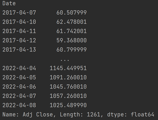
The price I will be using is Adjusted close price, it provide a fair way to compare performance of different stocks.

print(tsla5y['Adj Close'])

Output:

and the data of year-to-date is:

tslaYTD = web.DataReader("TSLA", "yahoo", thisYear, today)
print(tslaYTD['Adj Close'])

Output:

The next step is to find the corresponding criteria I have mentioned earlier:

i. Find Return since 2022-1-1 (%) (Year-to-Day)

(to convert into percentage, we divide last data by the first data to represent the ”percentage” of the first data)

# create new column to store the percentage change
tslaYTD['YTD Return'] = tslaYTD['Adj Close'] / tslaYTD['Adj Close'][0]
print(tslaYTD['YTD Return'])

Output:

for Tesla, the YTD percentage change is (0.970391-1) = -0.0296 = -2.96%

Since I only want a numeric value, the data for each date is not that important, I can extract the item by the following:

# tail(1) get the last row, head(1) get the first row,item() return the value stored, round() to limit result to 2dp
tslaYTDReturnPercentage = round((tslaYTD['YTD Return'].tail(1).item() / tslaYTD['YTD Return'].head(1).item() - 1) * 100, 2)
print(tslaYTDReturnPercentage)

Output:

ii. Return since 2017-4-8 (%) (5 years return)

# to get 5y percentage return of Tesla
tsla5yReturnPercentage = round(((tsla5y['Adj Close'].tail(1).item() / tsla5y['Adj Close'].head(1).item()) - 1.0) * 100, 2)
print(tsla5yReturnPercentage)

Output:

iii. Max Return (%) (5 years)

To find the maximum return in percentage we can us max() to find out the max value over the given period, then use it to calculate the percentage.

# find max return - use the max price occurred in the time period to calculate the percentage
tsla5yMR = round(((tsla5y['Adj Close'].max() / tsla5y['Adj Close'].head(1).item()) - 1.0) * 100, 2)
print(tsla5yMR)

Output:

iv. Max Drawdown(%) (5years)

This one is tricky to find, because I need to dynamically look for the greatest percentage change from high price (record high at that date) to low price, the “first-day-price” is not that important. In order to find out MDD, we need to use cummax() and cummin() to dynamically analyse the data set.

# find MDD
roll_max = tsla5y['Adj Close'].cummax()
print(roll_max)
daily_draw_down = tsla5y['Adj Close']/roll_max - 1.0
print(daily_draw_down)
max_draw_down = daily_draw_down.cummin()
print(max_draw_down)

# conclusion
print(round(max_draw_down.tail(1).item() * 100, 2))

Variable	Purpose	Output
roll_max (also know as record high)	check current price with current_max price, price of the date will be replaced by the record high up to that date. in the end the data will be the highest within the period.
daily_draw_down (daily % lower than the record high up to that day)	once we have the roll_max, we can divide daily data by roll_max of the same day to get the “daily draw down with respect to the record roll_max up to that date”
max_draw_down	find out the “maximum” (most negative) of daily_draw_down value and carry it forward
Conclusion:

Part B - Make it Systematic – functions call

Since I am going to perform same task for other stocks (AAPL, NVDA, SHOP and BAC),

I then write the code into functions and make it reusable:

The program's duty:

1. The “main” function allow user to input a valid ticker (program will fail if the user enter an invalid ticker)

2. It passes the ticker string to Pandas Datareader to create useful dataframe objects.

3. Each dataframe is passed to respective functions to calculate the value in my criteria.

4. All the value is stored in dictionary (key:value pair) and the dictionary is printed to terminal

(in the dictionary, the value is in list type “[]” for integrating with database in the next part)

part_B_stock_stat_gen.py

import pandas_datareader.data as web
import datetime
import pandas as pd

pd.set_option('display.max_rows', 40)
pd.set_option('display.max_columns', 10)
pd.set_option('display.width', 1000)
fiveYearAgo = datetime.datetime(2017, 4, 8)
thisYear = datetime.datetime(2022, 1, 1)
today = datetime.datetime(2022, 4, 8)


def cal_percentage_return(stock):
    return round(((stock['Adj Close'].tail(1).item() / stock['Adj Close'].head(1).item()) - 1.0) * 100, 2)


def cal_max_return_5y(stock5y):
    stock5y_mr = round(((stock5y['Adj Close'].max() / stock5y['Adj Close'].head(1).item()) - 1.0) * 100, 2)
    return stock5y_mr


def cal_mdd_5y(stock5y):
    roll_max = stock5y['Adj Close'].cummax()
    daily_draw_down = stock5y['Adj Close'] / roll_max - 1.0
    max_draw_down = daily_draw_down.cummin()
    return round(max_draw_down.tail(1).item() * 100, 2)


def load_ticker(stock_ticker):
    stock_ytd = web.DataReader(stock_ticker, "yahoo", thisYear, today)
    stock5y = web.DataReader(stock_ticker, "yahoo", fiveYearAgo, today)
    stock_ytd_return_percentage = cal_percentage_return(stock_ytd)
    stock5y_return_percentage = cal_percentage_return(stock5y)
    stock_max_return_5y = cal_max_return_5y(stock5y)
    stock_mdd_5y = cal_mdd_5y(stock5y)
    stock_stat = {
        "Ticker": [stock_ticker],
        "YTD Return": [stock_ytd_return_percentage],
        "5 Year Return": [stock5y_return_percentage],
        "Max Return(5Year)": [stock_max_return_5y],
        "Max Drawdown(5Year)": [stock_mdd_5y],
        "Weighed Score": [round(
            stock_ytd_return_percentage * 15 + stock5y_return_percentage * 5 + stock_max_return_5y * 1 + stock_mdd_5y * 30)]
    }
    return stock_stat


if __name__ == '__main__':
    ticker_input = ""
    while ticker_input != "exit":
        ticker_input = input('Enter the Stock ticker you wanna analyse ( "exit" to exit):')
        if ticker_input != "exit":
            print(load_ticker(ticker_input))

Output:

Conclusion: Tesla score the most under my criteria (8043), it is consider to be best-fit of my risk-reward requirement.

Part C - Populate Result into Database

The analysis result is naturally in tabular format, the next step is to store the result into database so that it can be manage easily.

First, I will create a new database by using MariaDB used in CPRG251 so that I do not need to make the whole thing from scratch/

part_C_01_mariadb_new_db.py

import sqlalchemy
import mariadb

# connect to database
engine = sqlalchemy.create_engine("mariadb+mariadbconnector://root:password@localhost:3306")

# create new data base called stock_analysis
engine.execute("CREATE DATABASE stock_analysis")

the terminal should not display any error msg, that indicate the new db has been created successfully.

if you run the same code the second time the following error msg will show up (As the database already exist):

Output:

Once the Database is created, we can further create table in it:

part_C_03_mariadb_stock_analysis_table_create.py

import pandas as pd
import sqlalchemy
import mariadb
from sqlalchemy import Table, Column, Integer, String, MetaData, Float

# connect to database
engine = sqlalchemy.create_engine("mariadb+mariadbconnector://root:password@localhost:3306/stock_analysis", echo=True)

meta = MetaData()

stock_stat = Table(
    'stock_statistic', meta,
    Column('Ticker', String(10), primary_key=True),
    Column('YTD Return', Float),
    Column('5 Year Return', Float),
    Column('Max Return(5Year)', Float),
    Column('Max Drawdown(5Year)', Float),
    Column('Weighed Score', Float)
)

meta.create_all(engine)

# read table and turn it into DataFrame type
table_df = pd.read_sql_table('stock_statistic', con=engine)
table_df.info()

P.S. the column name should match the key in the dictionary we created in previous program

Output:

Once the table is created we can insert testing data to test it:

part_C_04_mariadb_stock_analysis_insert_test.py

import pandas as pd
import sqlalchemy
import mariadb
pd.set_option('display.max_rows', 40)
pd.set_option('display.max_columns', 10)
pd.set_option('display.width', 1000)

from sqlalchemy import Table, Column, Integer, String, MetaData, Float

# connect to database
engine = sqlalchemy.create_engine("mariadb+mariadbconnector://root:password@localhost:3306/stock_analysis", echo=True)

test_data = {
    "Ticker": ['test'],
    "YTD Return": [1.0],
    "5 Year Return": [2.0],
    "Max Return(5Year)": [3.0],
    "Max Drawdown(5Year)": [4.0],
    "Weighed Score": [5.0]
}

test_data_df = pd.DataFrame.from_dict(test_data)
test_data_df.to_sql('stock_statistic', con=engine, if_exists='append', chunksize=1000, index=False)
print(pd.read_sql("SELECT * FROM stock_statistic", con=engine))

Output:

Part D - Put them all together and scale it up

Now I have the database for storing the statistic data. The final thing I want to do is to make a program not only calculating the criteria but also populating the result to the table.

Requirements for my program:

Once the program is running, it will ask me to enter a valid ticker to start analyse, OR "print" to list the stock_statistic table (alphabetically) OR "printmax" to list the stock_statistic table (order by Weighed Score) OR "maxonly" to list the entry in the stock_statistic table having highest Weighed Score OR "del "+ticker to delete existing entry with corresponding ticker e.g. "del tsla" OR "exit" to exit the program
It is capable of doing SELECT, INSERT and DELETE operation to the table.
If user input is a valid ticker, the program will print the stock stat in dictionary format in terminal, meanwhile inserting the stat into “stock_statistic”.
Basic error handling

P.S. the program needs to handle “RemoteDataError” if no data is fetched from DataReader method.

P.S. in the current design the date is fixed, that is enough for me to analyse different stock in an fair manner, in the future version I will make the time period to be dynamically changing so the data retrieved will always be “Past 5 years” and “YTD (up to TODAY)

P.S.The table structure is current accepting each ticker once only (because it is the primary key), it make sense to the current design since the “time period” is fixed, the same ticker will always have the same stat, so there is no need to allow the statistic for the same stock.

Following is the video walk-through of me creating the program base on the requirement.

https://youtu.be/bMW0ZZGQHCU

After my program is done I have entered 50 stocks into the table out of curiosity, following is the result (some of them do not have 5-year long data so the score might not be "fair" among them) :

Conclusion:

After finishing the project I can really feel the power of Python in the data science field. There are so many great resources online to learn Python. If you are interested in stock analysis you could also tweak the parameter and make your own program! There are also further steps that can be done, such as connecting the result with trading platform API to make automatic trade base on your own conditions (ALGO trade) or use the graph plotting function to do a technical analysis. I hope the two blogs together can bring something to the table.

BONUS:

Getting numerical data is sometimes not enough for analysing, we also need to plot them into a graph. we can import matplotlib to do so.

bonus_1_plot_graph.py

import pandas_datareader.data as web
import datetime
import pandas as pd
import matplotlib.pyplot as plt
pd.set_option('display.max_rows', 40)
pd.set_option('display.max_columns', 10)
pd.set_option('display.width', 1000)
fiveYearAgo = datetime.datetime(2017, 4, 8)
today = datetime.datetime(2022, 4, 8)

tsla5y = web.DataReader("TSLA", "yahoo", fiveYearAgo, today)


tsla5y['Adj Close'].plot(figsize=(32, 9))
plt.title('Tesla Stock Price')
plt.ylabel('Adjusted Closing Price')
plt.grid(color='grey', linestyle='--', linewidth=0.5)
plt.show()

Once the program run there is a window popped up, show the plot of adjusted close price against date.

Output:

Also Pandas Datareader supports reading data from multiple sources, for example:

bonus_2_other_source.py

import pandas_datareader.data as web
import datetime
import pandas as pd
import matplotlib.pyplot as plt
pd.set_option('display.max_rows', 40)
pd.set_option('display.max_columns', 10)
pd.set_option('display.width', 1000)

fiveYearAgo = datetime.datetime(2017, 4, 8)
today = datetime.datetime(2022, 4, 8)

# https://fred.stlouisfed.org/series/CPIAUCSL the link is the source
# Consumer Price Index for All Urban Consumers: All Items in U.S. City Average
cpi = web.DataReader("CPIAUCSL", "fred", fiveYearAgo, today)
print(cpi)

# https://fred.stlouisfed.org/series/LRUNTTTTCAM156S
# Unemployment Rate: Aged 15 and Over: All Persons for Canada
unemp_rate = web.DataReader("LRUNTTTTCAM156S", "fred", fiveYearAgo, today)
print(unemp_rate)

cpi.plot()
unemp_rate.plot()
plt.show()

Reference

T. kubheka. “Stock Market Analysis Using Python Pandas”, Level Up Coding, December 20, 2021. [Online] Available: https://levelup.gitconnected.com/stock-market-analysis-using-python-pandas-ec278f76e217 [Accessed: April 1, 2022]

V. Tatan. “In 12 minutes: Stocks Analysis with Pandas and Scikit-Learn”, Towards Data Science, May 27, 2019. [Online] Available:https://towardsdatascience.com/in-12-minutes-stocks-analysis-with-pandas-and-scikit-learn-a8d8a7b50ee7[Accessed: April 3, 2022]

Rune “Pandas for Financial Stock Analysis”, learn python with rune, May 6, 2021. [Online] Available:https://www.learnpythonwithrune.org/pandas-for-financial-stock-analysis/[Accessed: April 5, 2022]

Disclaimer:

The Content is for informational purposes only, you should not construe any such information or other material as legal, tax, investment, financial, or other advice.

This article was made purely as the author’s side project and in no way driven by any other hidden agenda.

Stock price analysis using Python with Pandas Library and SQL

Introduction:

Which stocks and which criteria am I going to compare?

Part A - Getting historical stock prices and Calculating criteria

Part B - Make it Systematic – functions call

Part C - Populate Result into Database

Part D - Put them all together and scale it up

Conclusion:

BONUS:

Reference

Recent Posts

Comments